Formatting and customization

Overview

When you export data from Qlik Sense through Qalyptus, tables are delivered without formatting (this is the normal Qlik Sense API behavior).
With Qalyptus, you can fully customize the look of your reports using Excel’s native formatting features.

This section shows you how to:

• Apply conditional formatting to tables and pivot tables (with static or dynamic columns).
• Repeat table header rows across pages when exporting to PDF.

Standard formatting

You can use all native Excel features to format the tables, pivot tables, and variables exported by Qalyptus.
This includes customizing table headers, aligning content, resizing columns and rows, and applying number, date, or percentage formats.

Formatting can be applied in two different ways:

• Whole object formatting:
  If you insert the entire table or pivot table as a single object, you can apply formatting directly to the full range of cells.
  For example, you can change the font style or font size.
  In this case, Qalyptus will automatically adjust the column width to fit the content.

Column-by-Column Formatting

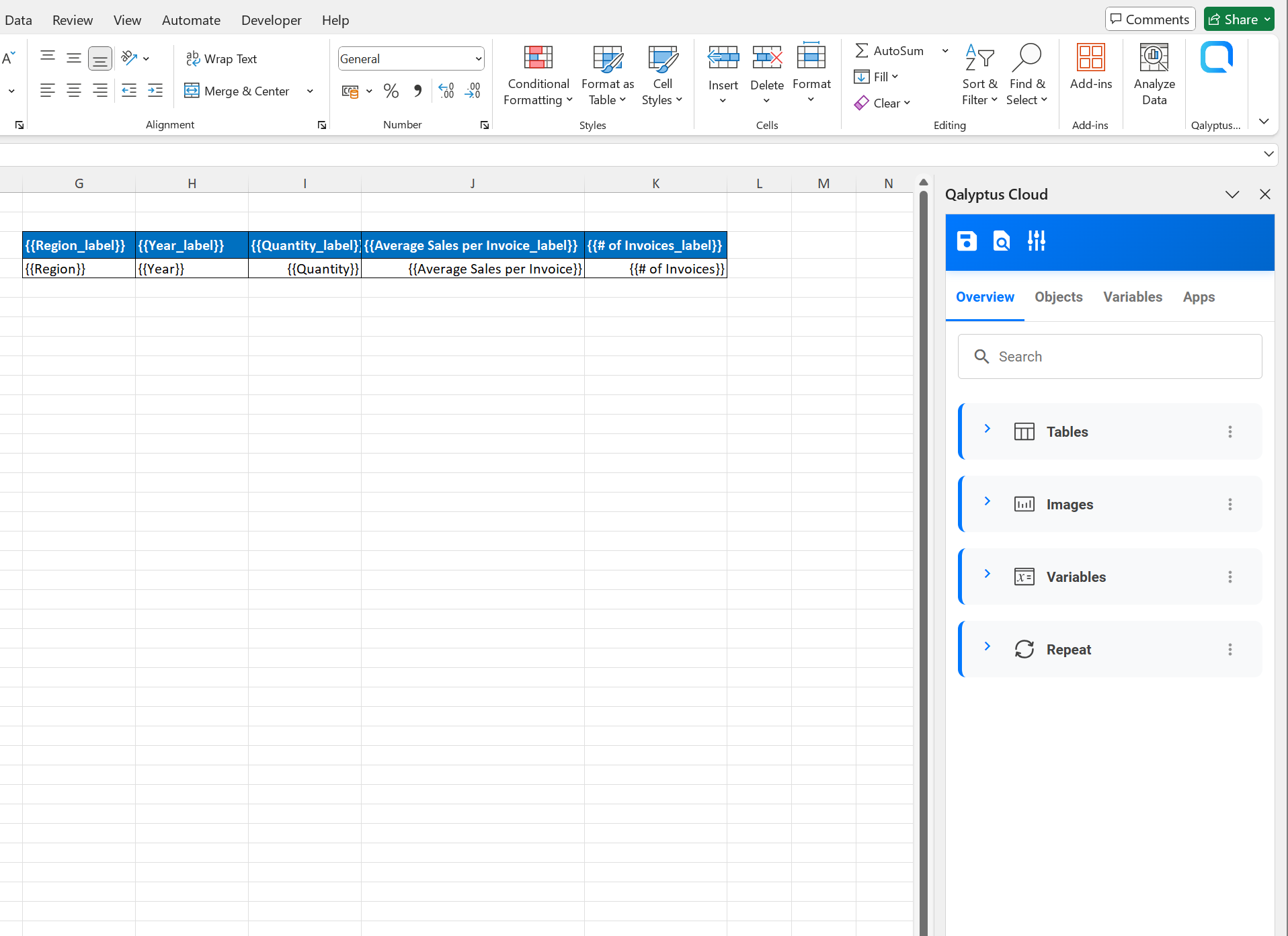
When you insert a table column, two rows are automatically generated:

• Header row: Contains the column title
• Data row: Contains a placeholder for the data

You can format each column's header and data independently, giving you complete control over the appearance of your tables. This flexibility allows you to:

• Apply different number formats (currency, percentage, decimals, etc.).
• Resize columns and rows.
• Left-align text columns, right-align numeric columns, and center-align dates for better readability.
• Customize fonts and styles per column.
• Percentage formatting to dsplay ratios or KPIs as percentages with one or two decimals.
• Date formatting to show dates in formats like dd/MM/yyyy, MM-dd-yyyy, or MMMM yyyy.
• and more.

How to Format Columns

1. Select the cell you want to format (either the header or data cell).
2. Apply formatting using Excel's formatting features.
3. The formatting will be applied as follows:
   • Header formatting is applied to the header in the generated report.
   • Data cell formatting is replicated to all cells in that column after report generation.

Conditional formatting

The table data is exported from Qlik Sense without formatting. In the Excel template, you can use the Conditional formatting feature to format tables exported from Qlik Sense apps.

In this section, we will see two different options to apply conditional formatting for tables and pivot tables.

1. Column-by-column formatting

If you choose to use a Qlik Sense table or Pivot table in Excel by dragging and dropping its columns, you can add a conditional format for each column.

This option allows you to apply different formats (text color, background color, text size, etc.) for each column.

To format a column, do the following:

• Insert the table or pivot table columns
• Select a data cell in the column to format
• Click Conditional Formatting
• Add one or more rules to format the column
• After generating the report, Qalyptus will format all the column values.

Here is a video showing an example of conditional formatting for a table column.

caution

Column-by-column formatting is possible only for a table object or a pivot table with static columns.
Static columns mean that the measure columns are not duplicated by using a dimension in the Column area.

You cannot use column-by-column formatting when the exported columns are dynamic and not known by Qalyptus in advance.

See the following image to learn more

caution

Adapt the Excel formula to your Excel localization settings.
The function names and the parameter separators may vary depending on your language and regional settings.

In the example above, Excel is configured in English, so the function names are in English and the parameters are separated by commas.

2. Dynamic formatting

This second method can be used to format a table or any pivot table, including pivot tables with static or dynamic columns.

To format a table or pivot table, do the following:

• Insert the table or pivot table shortcode
• Select the cell that contains the shortcode
• Click Conditional Formatting
• Click New Rule...
• Select the rule type: Use a formula to determine which cells to format
• Add a formula to format table columns and rows
• Choose the cell format to apply when the condition is met

Here is an example formula:

=(ROW()>=8)*(COLUMN()>=3)*(INDIRECT(ADDRESS(ROW(),COLUMN()))>1000)*(INDIRECT(ADDRESS(ROW(),COLUMN()))<>"-")

In the following example, we will format a pivot table that cannot be formatted with the first method (column-by-column formatting).

The columns of the pivot table are dynamic and can change when the Year field values change.

tip

Here are some useful functions you can use in a conditional formatting formula:

• ROW(): Returns the row number
• COLUMN(): Returns the column number
• INDIRECT(ADDRESS(ROW(),COLUMN())): Returns the current cell reference
• Use the asterisk symbol * as the AND operator

caution

Adapt the Excel formula to your Excel localization settings.
The function names and the parameter separators may vary depending on your language and regional settings.

In the example above, Excel is configured in English, so the function names are in English and the parameters are separated by commas.

Repeat table header row across pages for a PDF

To repeat the table header on all pages when you have a large table, drag and drop the columns of the table object, then:

1. In Excel, click the Page Layout tab
2. In the Page Setup group, click Print Titles
3. Under the Sheet tab, click the icon on the right of the Rows to repeat at top field
4. Select the row you want to appear at the top of every page, then press Enter
5. Click OK

Here is the result: