Excel report

Overview

This section will create an Excel report using Qlik Sense objects.

To create an Excel report, go to the Reports tab and click Create report button.

1. Give a name to your report
2. Add a description if you wish (optional)
3. In the Type drop-down menu, select Excel
4. Select a project
5. Click Save

You will be redirected to the report Overview tab. In the Template field, click the Edit button. An Excel file will be downloaded.

1. Open the Excel file

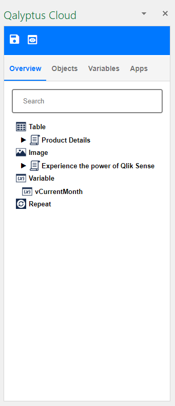
2. The Qalyptus Cloud Office add-in will be automatically open in the task pane. If you use Office for the web, click the add-in icon to open it.

3. The Apps tab lists all your Qlik Sense apps. You can select one or more apps to use to create the report. After choosing an app, click on the three-point button to refresh its metadata (variables, objects, and fields)

4. The Variables tab lists the Qlik variables of the selected apps. Select the ones you want to use

5. The Objects tab lists the Tables, Charts, and Master Items of the selected apps. Select the ones you want to use

6. The Overview tab shows selected objects and variables to use in your template

7. The Save button allows you to save the template file

8. The Preview button allows you to have a preview of the report

   

Add objects to the template file

Let's create a simple template using a chart, a table, and a variable.

1. Select the Apps tab and choose a Qlik Sense app
2. In the Variables tab, right-click on a variable and select Add variable
3. In the Objects tab, find the chart you want to use, right-click, and choose Use object as an image. Find the object table you wish to use, right-click, and select Use ** object as table**
4. Select the Overview tab to insert the object into the file
5. Before inserting an item, don't forget the select the destination cell
6. Under the Variables node, right-click on the variable previously added and choose Insert
7. Under the Table node, right-click on the table object previously added, and select Insert or Insert columns. The first option will use the whole object, which will be exported as it is in Qlik Sense? The second one will allow you to format each column of the table using the Excel features
8. Under the Image node, right-click on the chart previously added and select Insert
9. You can use all the Excel features to format the file: resize the chart image, format the table columns, add additional text and images, etc.
10. Click Preview to see the result
11. Click Save to save the file. You can close the file and back to Qalyptus Cloud

Conditional formatting

The table data is exported from Qlik Sense without formatting (normal Qlik Sense API behavior). In the Excel template, you can use the Conditional formatting feature to format the tables exported from the Qlik Sense apps.

In this section, we will see two different options to apply conditional formatting for tables and pivot tables.

1. Column-by-column formatting

If you choose to use a Qlik Sense table or Pivot table in Excel by dragging and dropping its columns, you can add a conditional format for each column.

This option allows you to apply different formats (text color, background color, text size, etc.) for each column.

To format a column, do the following:

• Insert the table or the pivot table columns
• Select a data cell in the column to format
• Click Conditional Formatting
• Add one or many rules to format the column
• After generating the report, Qalyptus will format all the column values.

Here is a video showing an example of conditional formatting for a table column.

caution

Column-by-column formatting is possible only to format a table object or a pivot table that has static columns. By static columns, we mean that the measure columns are not duplicated by using a dimension to the Column area.

You cannot use the column-by-column formatting when the exported columns are dynamic and are not known by Qalyptus in advance.

See the following image to learn more

2. Dynamic formatting

This second method can format a table and any pivot table, a pivot table with static or dynamic columns.

To format a table or a pivot table, do the following:

• Insert the table or the pivot table shortcode
• Select the cell that contains the shortcode
• Click Conditional Formatting
• Click New Rule...
• Select the rule type: Use a formula to determine which cells to format
• Add a formula to format table columns and rows
• Choose the format of the cell to apply when the condition is verified

Here is an example of a formula:

=(ROW()>=8)*(COLUMN()>=3)*(INDIRECT(ADDRESS(ROW(),COLUMN()))>1000)*(INDIRECT(ADDRESS(ROW(),COLUMN()))<>"-")

In the following example, we will format a pivot table that cannot be formatted with the first method (Column by column formatting).

The columns of the pivot table are dynamic and can change when the Year field values change.

tip

Here are some useful functions that you can use in a conditional formatting formula:

• ROW(): Row number
• COLUMN(): Column number
• INDIRECT(ADDRESS(ROW(),COLUMN()): Current cell reference
• Use the star symbol (*) for the AND operator

Add a filter to an object

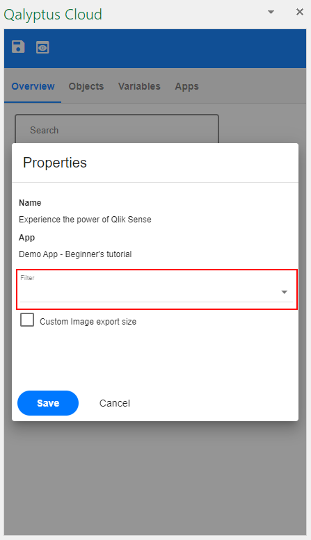
In addition to applying filters at the task level, you can apply a filter for each Qlik object you use in your template.

Right-click on the object to which you want to add a filter, and select Properties. In the Properties screen, select the filter to apply from the filter list. Only one filter can be applied to an object.

Not insert new rows option

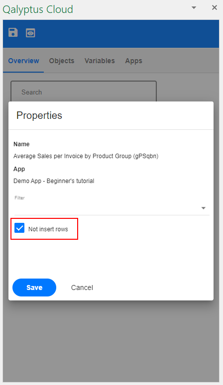
When you use an object as a table, by default, Qalyptus inserts new rows to keep the same layout of your different objects. But in some cases, you may want Qalyptus not to insert rows, for example, when you have several objects next to each other.

You have the option of not inserting rows when exporting a table.

Right-click on a table or pivot table object, and select Properties. In the Properties screen, check the checkbox Not insert rows.

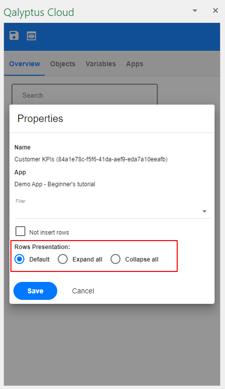
Choose pivot table rows presentation

You can choose how you want to export a pivot table. You can choose Default (the settings selected in Qlik Sense), Extend all, or Collapse all.

Export an object with a different size

When you want to use a Qlik Sense object (chart or table) as an image in your report template, drag and drop the object to the template file. Qalyptus will create a placeholder image that you can resize. When you generate the report, Qalyptus will export the Qlik Sense object with the dimension of the placeholder image and put it in the placeholder image.

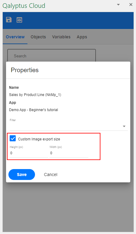
It is possible to export the image with a large or small size as the placeholder image size. For example, export the image 1200 x 800 px and use it in the size 1000 x 600 px file.

Select the option Custom export dimensions in the object Properties, then enter the Height and Width value.

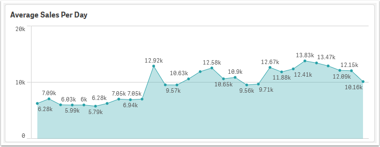
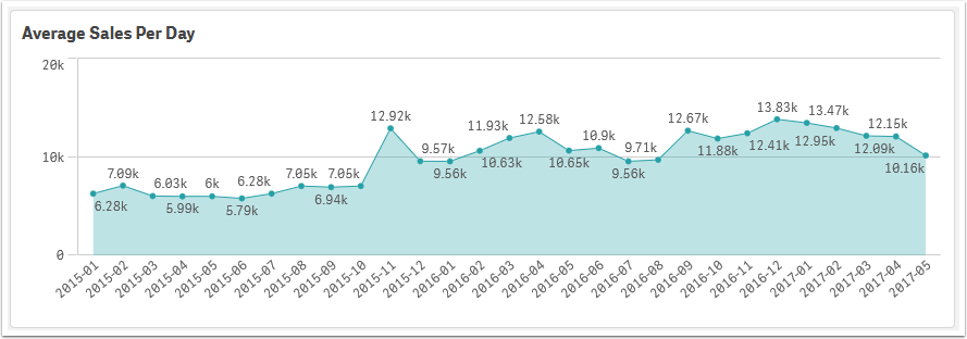
Exporting an object with a large size allows you to get more information; Qlik Sense can hide some information when you reduce the size.

Chart with a small size (export size = size of use )

The same chart with a large export size (export size > size of use )

Create native Excel PivotTable

Qalyptus allows you to generate native Excel PivotTables in your reports using data exported from a Qlik Sense table.

To create a PivotTable, follow these steps.

1. Insert Qlik Sense table columns into your Excel template
   In your Excel template:

   • Insert individual columns from your Qlik Sense table into a worksheet.
   • Do not insert the whole object tag — this is not supported for PivotTables.

2. Important: Column headers must not contain Qalyptus tags
   The header row of your data source must not contain any Qalyptus tags (such as {{Sales_label}}).
   For example, use: Sales instead of {{Sales_label}}.

3. Add an empty row at the end of the data source range
   To ensure the PivotTable works correctly during report generation, include an empty row after your data.

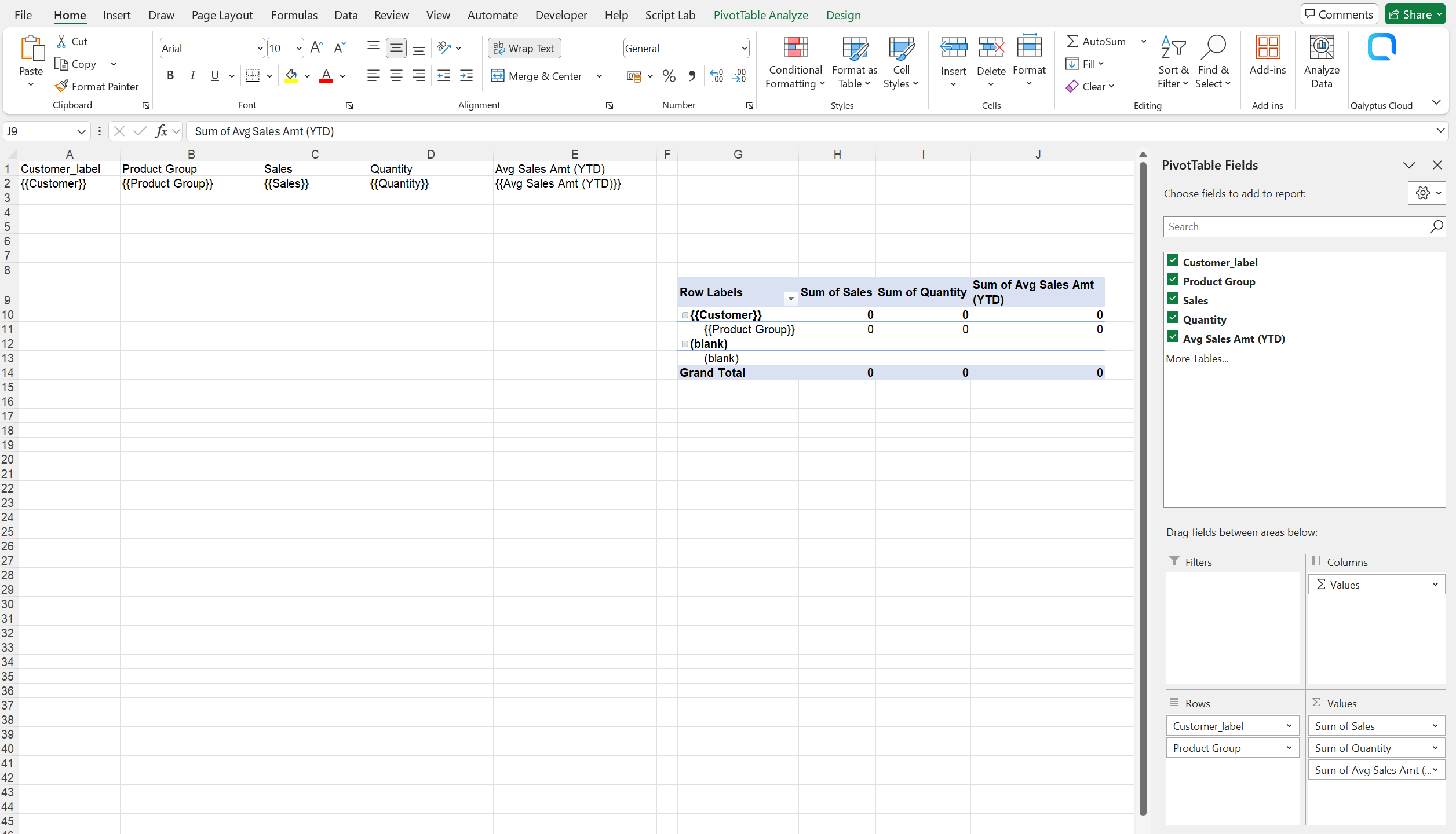
4. Create the PivotTable

• Select the data range (including the empty row).
• Go to Insert → PivotTable.
• Place the PivotTable on a new worksheet or in the same one.

5. Configure the PivotTable
   Use Excel's PivotTable options to define your rows, columns, filters, and values as needed.

6. Preview Return to the Qalyptus Cloud Office add-in and click the Preview button to see the result.

tip

You can hide the sheet that contains the PivotTable's data source to keep your final report clean and focused on the result.

Export Images and URLs in Excel Reports

Qalyptus supports exporting URLs and images from Qlik Sense tables into Excel and PDF reports.

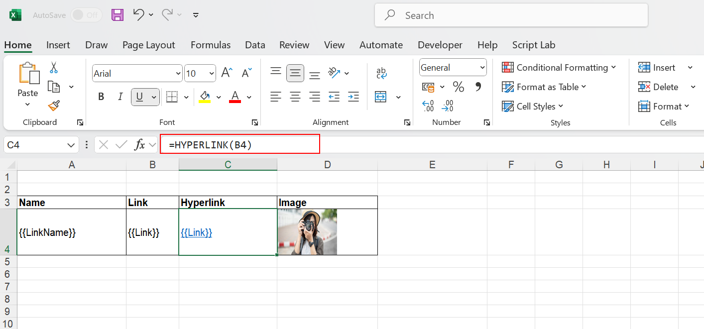
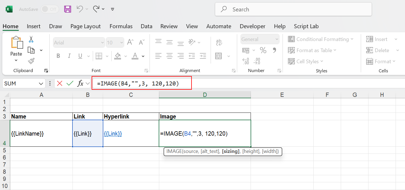
• For URLs, use the Excel formula HYPERLINK() to transform plain URLs into clickable hyperlinks in Excel and PDF reports.
• For images, use the Excel formula IMAGE() to display them inside Excel cells and make them visible in generated reports.

The source parameter in the HYPERLINK() and IMAGE() functions must reference a cell within the table that will contain a URL once the report is generated. You can hide this column for better clarity.

info

Using formulas gives you more control over how hyperlinks appear and how images are sized within cells.

tip

You can hide the column that contains the hyperlink or image source URL.

Use Excel formulas

Qalyptus supports formulas on columns — for example, calculating totals using SUM().

To use a formula, you need to include at least the data cell and one additional cell, as shown below.
The row containing the additional cell can be hidden to keep the report clean and professional.

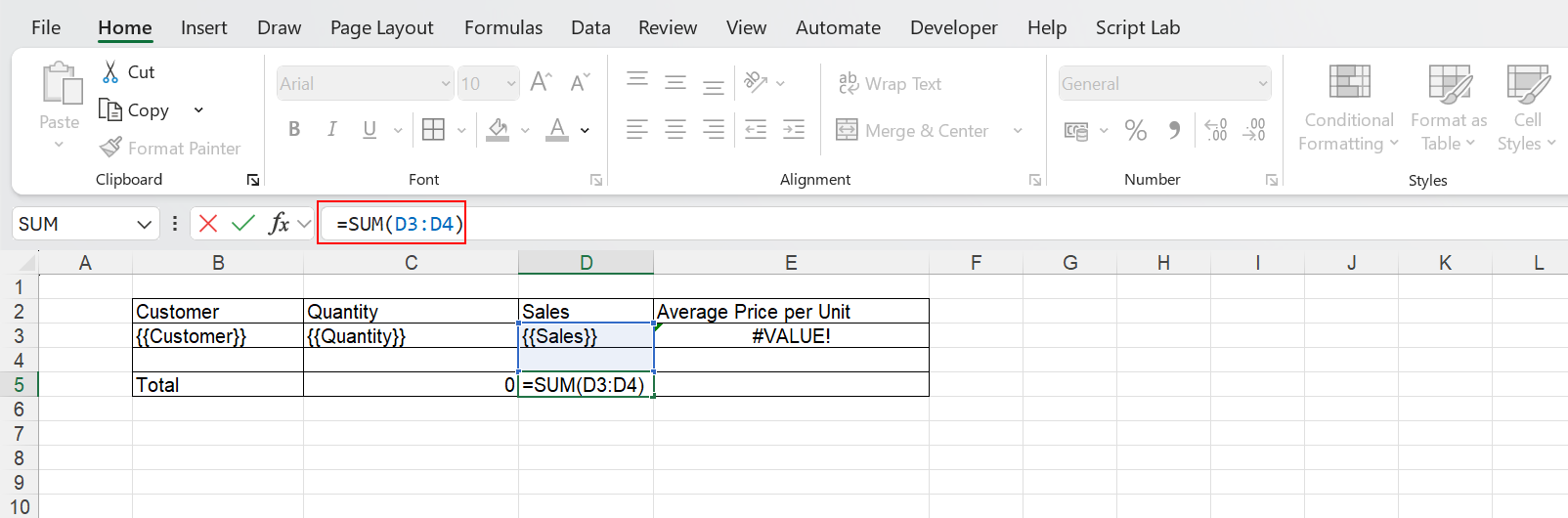
You can also apply formulas on rows.
For instance, you can calculate the Average Price per Unit using the formula: Sales / Quantity.

warning

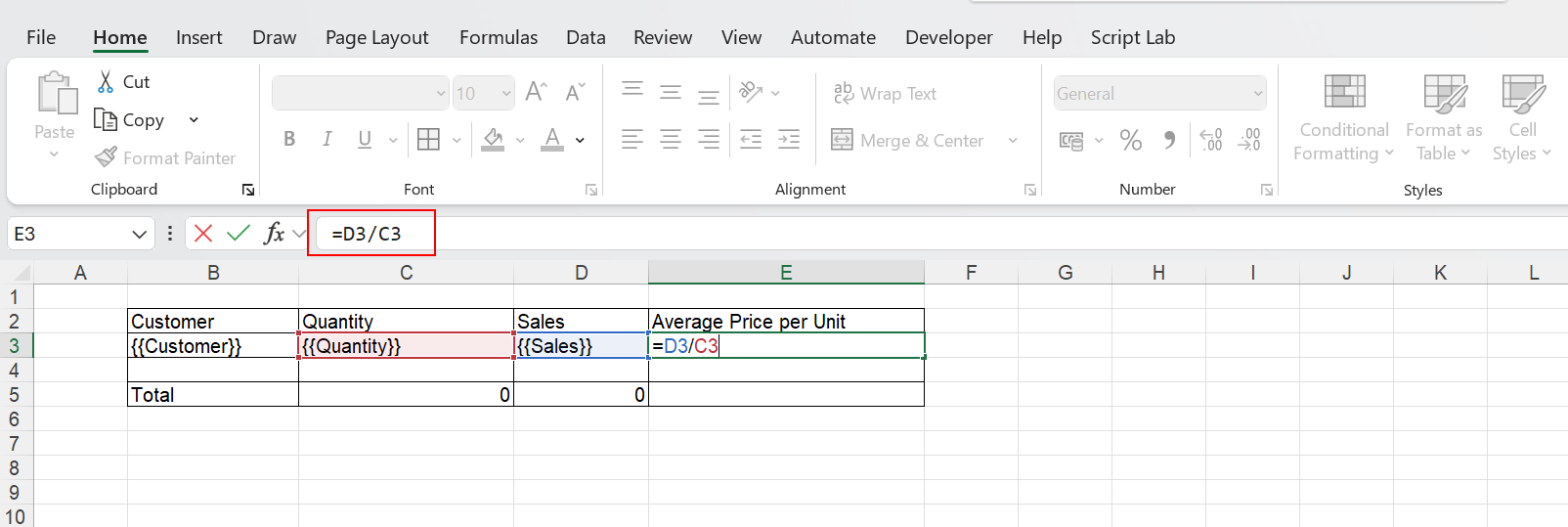
Formulas on rows must be placed in columns that are directly adjacent to the table columns.

Repeat on same sheet or across multiple sheets

Qalyptus allows repeating data by dimension in a report. You can repeat Images, Tables, and Variables.

You can repeat the same sheet's contents for each value in a dimension field. You can also repeat your Qlik Sense objects on a single sheet for a field value. You can nest the repeat levels as many times as you want.

See how you can do it.

note

The video uses Qalyptus Desktop; it works the same way with Qalyptus Cloud. We will produce a video with Qalyptus Cloud as soon as possible.

Repeat table header row across pages for a PDF

To repeat the first row of column headers on all pages when you have a large and complex worksheet, drag and drop the columns of the table object then:

1. In Excel, click the Page Layout tab
2. In the Page Setup group, click Print Titles
3. Under the Sheet tab, click on the icon on the right in the Rows to repeat at top field.
4. Select the row you wish to appear at the top of every page. Press the Enter key
5. Then click OK

Here is the result: